Battery Life Estimation#
This tutorial demonstrates estimation of how long a system can operate from a battery. sysLoss does not include battery models as such but can interface with user supplied battery models using callback functions. We will revisit the Bluetooth sensor from the first tutorial and evaluate the battery life with different battery models.
from sysloss.components import *
from sysloss.system import System
import numpy as np
import matplotlib.pyplot as plt
System definition#
The Bluetooth Sensor System is reused, including load phases, with the addition of 2D interpolation data for converter efficiency. The system is powered by a rechargeable lithium battery with a capacity of 156mAh and nominal voltage of 3.6V. Battery voltage varies a lot depending on state-of-charge (SOC), so converter efficiencies should reflect this.
CAPACITY = .156 # battery capacity in Ah
VNOMINAL = 3.6 # nominal battery voltage (V)
buck_eff = {"vi": [3.0, 5.0], "io": [1e-6, 1e-5, 1e-4, 1e-3, 1e-2], "eff": [[0.72, 0.89, 0.92, 0.925, 0.93],[0.65, 0.84, 0.87, 0.9, 0.91]]}
boost_eff = {"vi": [3.0, 4.5], "io": [1e-6, 1e-5, 1e-4, 1e-3, 1e-2], "eff": [[0.55, 0.65, 0.72, 0.8, 0.85],[0.62, 0.72, 0.81, 0.85, 0.91]]}
bts = System("Bluetooth sensor", Source("LiPo battery", vo=VNOMINAL, rs=0.0))
bts.add_comp("LiPo battery", comp=Converter("Buck 1.8V", vo=1.8, eff=buck_eff))
bts.add_comp("Buck 1.8V", comp=PLoad("MCU", pwr=13e-3))
bts.add_comp("LiPo battery", comp=Converter("Boost 5V", vo=5.0, eff=boost_eff, iis=3e-6))
bts.add_comp("Boost 5V", comp=RLoss("RC filter", rs=6.8))
bts.add_comp("RC filter", comp=ILoad("Sensor", ii=6e-3))
bts_phases = {"sleep": 3600, "acquire": 2.5, "transmit": 2e-3}
bts.set_sys_phases(bts_phases)
bts.set_comp_phases("Boost 5V", phase_conf=["acquire"])
mcu_pwr = {"sleep": 12e-6, "acquire": 15e-3, "transmit": 35e-3}
bts.set_comp_phases("MCU", phase_conf=mcu_pwr)
Ideal battery#
We start with an ideal battery. Although not invented yet, it has a constant output voltage and zero internal resistance. The battery life is then simply the battery capacity divided by average system current.
bdf = bts.solve()
bdf.tail()
| Component | Type | Parent | Phase | Vin (V) | Vout (V) | Iin (A) | Iout (A) | Power (W) | Loss (W) | Efficiency (%) | Warnings | |
|---|---|---|---|---|---|---|---|---|---|---|---|---|
| 17 | Sensor | LOAD | RC filter | transmit | 0.0 | 0.0 | 0.0 | 0.0 | 0.0 | 0.0 | 100.0 | |
| 18 | Buck 1.8V | CONVERTER | LiPo battery | transmit | 3.6 | 1.8 | 0.010522 | 0.019444 | 0.037879 | 0.002879 | 92.4 | |
| 19 | MCU | LOAD | Buck 1.8V | transmit | 1.8 | 0.0 | 0.019444 | 0.0 | 0.035 | 0.0 | 100.0 | |
| 20 | System total | transmit | 0.010525 | 0.03789 | 0.00289 | 92.373662 | ||||||
| 21 | System average | 0.000017 | 0.000062 | 0.000018 | 46.742804 |
# divide by 24 to get battery life in days
int(CAPACITY / (bdf[bdf.Component == "System average"]["Iout (A)"].values[0] * 24))
380
The ideal battery should provide power for 380 days. We can make callback functions for the .batt_life() method for an ideal battery as well, and run the battery life simulation.
Note
If the system has load phases, the battery is depleted by looping through the phases in the order they are defined.
cap = CAPACITY

def probe():
    """The probe function returns the current state of the battery"""
    global cap
    return (cap, VNOMINAL, 0.0)

def deplete(t, curr):
    """The deplete function depletes the battery with a current of duration t"""
    global cap
    cap -= t * curr / 3600.0
    if cap < 0.0:
        cap = 0.0
        return (0.0, 0.0, 0.0)
    return (cap, VNOMINAL, 0.0)

bldf = bts.batt_life("LiPo battery", cutoff=3.0, pfunc=probe, dfunc=deplete)
The output of the depletion process is a DataFrame with all the time steps of the simulation. The “Time (s)” column is the accumulated time, and the last row then holds the battery life in seconds.
bldf.tail()
| Time (s) | Capacity (Ah) | Voltage (V) | Resistance (Ohm) | |
|---|---|---|---|---|
| 27360 | 3.285482e+07 | 0.000029 | 3.6 | 0.0 |
| 27361 | 3.285842e+07 | 0.000022 | 3.6 | 0.0 |
| 27362 | 3.285842e+07 | 0.000012 | 3.6 | 0.0 |
| 27363 | 3.285842e+07 | 0.000012 | 3.6 | 0.0 |
| 27364 | 3.286202e+07 | 0.000005 | 3.6 | 0.0 |
int(bldf["Time (s)"].values[-1]/(24*3600))
380
The simulation agrees with the first calculation: 380 days.
Simple battery model#
The ideal battery model is generally too optimistic. We want to add voltage variation as a function for charge level and add some internal resistance. Also, most lithium batteries have a PCM (Protection Control Module) that draws a little current, plus there is self-discharge which is typically a few percent per month. To take these effects into account, we create a battery class.
class LiPo:
    def __init__(self, capacity, nom_volt, resistance, cutoff):
        self.capacity = capacity # Ah
        self.depleted = 0.0 # Ah
        self.rs = resistance # ohm
        self.nom_volt = nom_volt # V
        self.beta = 0.75 # adapt to battery
        self.k1 = 0.01 # adapt to battery
        self.k2 = 0.00003 # adapt to battery
        self.cutoff = cutoff # V
        self.pcm_curr = 1e-6 # protection circuit module (PCM) current
        self.dc_per_month = 0.05 # 5% self-discharge per month

    def calc_res(self):
        return self.rs

    def calc_ocv(self):
        soc = (self.capacity - self.depleted)/self.capacity
        if soc > 0.0:
            ocv = self.nom_volt + self.beta * (soc - 0.5) - self.k1 / soc + self.k2 / (1.001 - soc)
            if ocv < self.cutoff:
                return 0.0
            return ocv
        return 0.0

    def probe(self):
        """Callback function"""
        return (self.capacity - self.depleted, self.calc_ocv(), self.calc_res())

    def deplete(self, t, i):
        """Callback function"""
        consumed = i * t
        pcm_loss = self.pcm_curr * t
        soc = (self.capacity - self.depleted)/self.capacity
        self_deplete = soc * self.dc_per_month * t / (30*24*3600)
        self.depleted = min(self.depleted + (consumed + pcm_loss + self_deplete)/ 3600.0, self.capacity)
        return self.probe()
Let’s run another battery life estimation with this simple battery model:
Note
The progress bar will stop before the full battery capacity is depleted if the cutoff voltage is reached.
batt = LiPo(CAPACITY, VNOMINAL, 0.1, 3.0)
bldf2 = bts.batt_life("LiPo battery", cutoff=3.0, pfunc=batt.probe, dfunc=batt.deplete)
int(bldf2["Time (s)"].values[-1]/(24*3600))
343
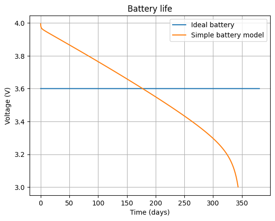
The estimated battery lifetime is now 343 days, down from 380 days on the ideal battery. We can now look at the battery voltage as a function of time:
Battery modelling with PyBaMM#
So far, the battery model hasn’t included the chemical reactions that occur inside the battery. Such battery models are complex, and the best option for including advanced battery models is to use a battery simulation package. PyBaMM (Python Battery Mathematical Modelling) is an open-source battery simulation package that sysLoss can interface with.
Start by installing PyBaMM.
%pip install pybamm -q
import pybamm
Next we define the two callback functions needed by the .batt_life() method. We select the parameter set “Ecker2015” that is a 156mAh battery.
model = pybamm.lithium_ion.DFN()
parameter_values = pybamm.ParameterValues("Ecker2015") # 156mAh model
parameter_values.update({"Current function [A]": "[input]"})
sim = pybamm.Simulation(model, parameter_values=parameter_values)
sim.step(1e-6, inputs={"Current function [A]":0.0}) # dummy step to initialize variables

def probe_pb():
    sol = sim.solution
    cap = parameter_values["Nominal cell capacity [A.h]"]
    return (cap - sol["Discharge capacity [A.h]"].entries[-1], sol["Voltage [V]"].entries[-1], sol["Local ECM resistance [Ohm]"].entries[-1])

def deplete_pb(t, curr):
    sim.step(t, solver=pybamm.CasadiSolver(mode="fast"), inputs={"Current function [A]":curr})
    return probe_pb()
If we tried .batt_life() with these callback functions and the Bluetooh sensor system, the simulation would take extremely long and probably fail. PyBaMM is not really made for year-long simulations, the default discharge rate is 1C. So, for a battery that would deplete in a matter of hours or perhaps a few days the PyBaMM callbacks could be used directly.
However, we can use the PyBaMM model to obtain voltage and resistance curves, which we can include in the battery class defined previoulsy. Let’s run the PyBaMM model with a discharge rate of 0.1C and 0.01C:
cap = parameter_values["Nominal cell capacity [A.h]"]
# 0.1C discharge
sim = pybamm.Simulation(model, parameter_values=parameter_values)
sim.solve([0,40000], initial_soc = 1.0, inputs={"Current function [A]": 0.1*cap})
sol_0c1 = sim.solution
# 0.01C discharge
sim = pybamm.Simulation(model, parameter_values=parameter_values)
sim.solve([0,400000], initial_soc = 1.0, inputs={"Current function [A]": 0.01*cap})
sol_0c01 = sim.solution
Let’s take a look at the battery voltage and resistance curves:
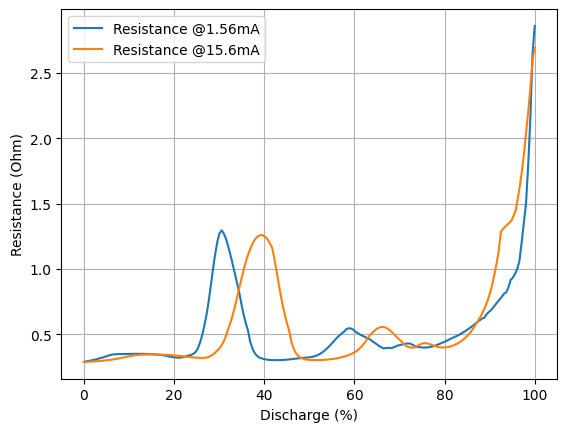
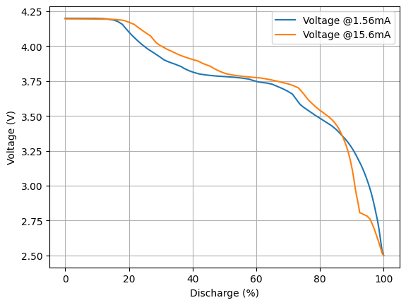
The curves are similar, so the 0.1C curves will be used in the battery class. A new class is made with updated methods for voltage and resistance calculations.
class LiPo2(LiPo):
    def calc_res(self):
        soc = (self.capacity - self.depleted)/self.capacity
        return np.interp(1.0 - soc, self.rs[0], self.rs[1])

    def calc_ocv(self):
        soc = (self.capacity - self.depleted)/self.capacity
        return np.interp(1.0 - soc, self.nom_volt[0], self.nom_volt[1])
Finally run .batt_life() with the updated battery class:
frx = sol_0c1["Local ECM resistance [Ohm]"].entries
fvx = sol_0c1["Voltage [V]"].entries
x = np.linspace(0.0, 1.0, len(frx), endpoint=True)
batt2 = LiPo2(cap, (x, fvx), (x, frx), 3.0)
bldf3 = bts.batt_life("LiPo battery", cutoff=3.0, pfunc=batt2.probe, dfunc=batt2.deplete)
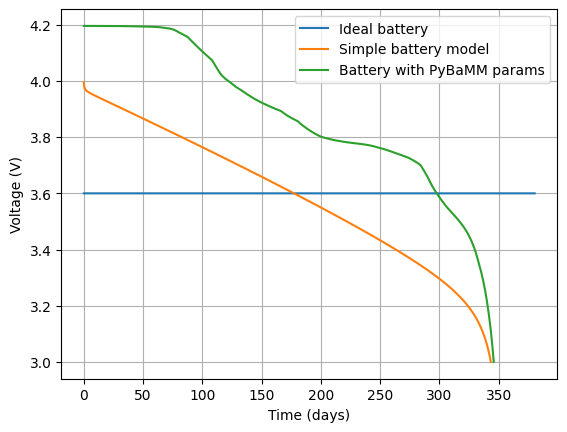
int(bldf3["Time (s)"].values[-1]/(24*3600))
345
The battery life estimate is now somewhat in the middle of the two previous estimates. Let’s look at the battery voltage for the three battery models:
Improve battery life#
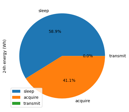
The current design will last for about a year. How can we improve the design to get longer battery life? Start by examining the energy consumed in each phase.
Tip
When the system is defined with load phases, the values in the “24h energy (Wh)” column are weighted with load phase duration. This allows direct comparison of energy consumption in different load phases.
bdf = bts.solve(energy=True)
bdf[bdf.Component == "System total"].plot.pie(y="24h energy (Wh)", labels=bdf.Phase.unique(), autopct='%1.1f%%');
---------------------------------------------------------------------------
ValueError                                Traceback (most recent call last)
Cell In[22], line 2
      1 bdf = bts.solve(energy=True)
----> 2 bdf[bdf.Component == "System total"].plot.pie(y="24h energy (Wh)", labels=bdf.Phase.unique(), autopct='%1.1f%%');

File ~/checkouts/readthedocs.org/user_builds/sysloss/envs/latest/lib/python3.11/site-packages/pandas/plotting/_core.py:1959, in PlotAccessor.pie(self, y, **kwargs)
   1953 if (
   1954     isinstance(self._parent, ABCDataFrame)
   1955     and kwargs.get("y", None) is None
   1956     and not kwargs.get("subplots", False)
   1957 ):
   1958     raise ValueError("pie requires either y column or 'subplots=True'")
-> 1959 return self(kind="pie", **kwargs)

File ~/checkouts/readthedocs.org/user_builds/sysloss/envs/latest/lib/python3.11/site-packages/pandas/plotting/_core.py:1185, in PlotAccessor.__call__(self, *args, **kwargs)
   1182             label_name = label_kw or data.columns
   1183             data.columns = label_name
-> 1185 return plot_backend.plot(data, kind=kind, **kwargs)

File ~/checkouts/readthedocs.org/user_builds/sysloss/envs/latest/lib/python3.11/site-packages/pandas/plotting/_matplotlib/__init__.py:71, in plot(data, kind, **kwargs)
     69         kwargs["ax"] = getattr(ax, "left_ax", ax)
     70 plot_obj = PLOT_CLASSES[kind](data, **kwargs)
---> 71 plot_obj.generate()
     72 plt.draw_if_interactive()
     73 return plot_obj.result

File ~/checkouts/readthedocs.org/user_builds/sysloss/envs/latest/lib/python3.11/site-packages/pandas/plotting/_matplotlib/core.py:518, in MPLPlot.generate(self)
    516 self._compute_plot_data()
    517 fig = self.fig
--> 518 self._make_plot(fig)
    519 self._add_table()
    520 self._make_legend()

File ~/checkouts/readthedocs.org/user_builds/sysloss/envs/latest/lib/python3.11/site-packages/pandas/plotting/_matplotlib/core.py:2181, in PiePlot._make_plot(self, fig)
   2177 # labels is used for each wedge's labels
   2178 # Blank out labels for values of 0 so they don't overlap
   2179 # with nonzero wedges
   2180 if labels is not None:
-> 2181     blabels = [
   2182         blank_labeler(left, value)
   2183         for left, value in zip(labels, y, strict=True)
   2184     ]
   2185 else:
   2186     blabels = None

File ~/checkouts/readthedocs.org/user_builds/sysloss/envs/latest/lib/python3.11/site-packages/pandas/plotting/_matplotlib/core.py:2181, in <listcomp>(.0)
   2177 # labels is used for each wedge's labels
   2178 # Blank out labels for values of 0 so they don't overlap
   2179 # with nonzero wedges
   2180 if labels is not None:
-> 2181     blabels = [
   2182         blank_labeler(left, value)
   2183         for left, value in zip(labels, y, strict=True)
   2184     ]
   2185 else:
   2186     blabels = None

ValueError: zip() argument 2 is shorter than argument 1
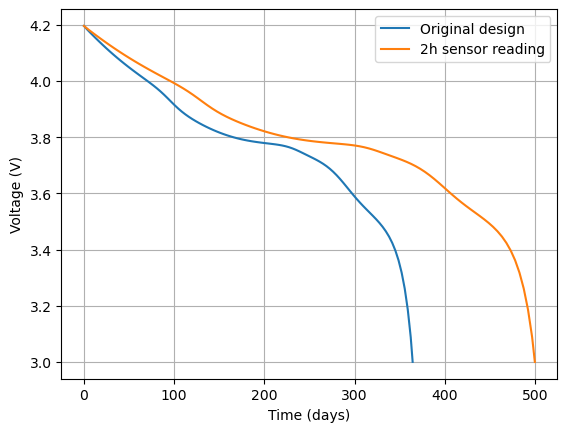
The acquire phase consumes the most energy. Let’s say it is acceptable to increase the sensor reading interval from 1 hour to 2 hours. That will save some energy - and now it is the sleep phase that consumes the most energy.
bts_phases = {"sleep": 7200, "acquire": 2.5, "transmit": 2e-3}
bts.set_sys_phases(bts_phases)
bdf2 = bts.solve(energy=True)
bdf2[bdf2.Component == "System total"].plot.pie(y="24h energy (Wh)", labels=bdf2.Phase.unique(), autopct='%1.1f%%');
batt2 = LiPo2(cap, (x, fvx), (x, frx), 3.0)
bldf4 = bts.batt_life("LiPo battery", cutoff=3.0, pfunc=batt2.probe, dfunc=batt2.deplete)
Battery life has been extended to about 500 days by increasing the sensor reading interval to 2 hours.
To address the energy consumption in the sleep phase, we could maybe shut down all peripherals in the MCU except for the timer and enable a deep sleep mode. Let’s say this reduces the MCU power from 12uW to 0.85uW.
mcu_pwr = {"sleep": 0.85e-6, "acquire": 15e-3, "transmit": 35e-3}
bts.set_comp_phases("MCU", phase_conf=mcu_pwr)
bdf3 = bts.solve(energy=True)
bdf3[bdf3.Component == "System total"].plot.pie(y="24h energy (Wh)", labels=bdf3.Phase.unique(), autopct='%1.1f%%');

batt2 = LiPo2(cap, (x, fvx), (x, frx), 3.0)
bldf5 = bts.batt_life("LiPo battery", cutoff=3.0, pfunc=batt2.probe, dfunc=batt2.deplete)
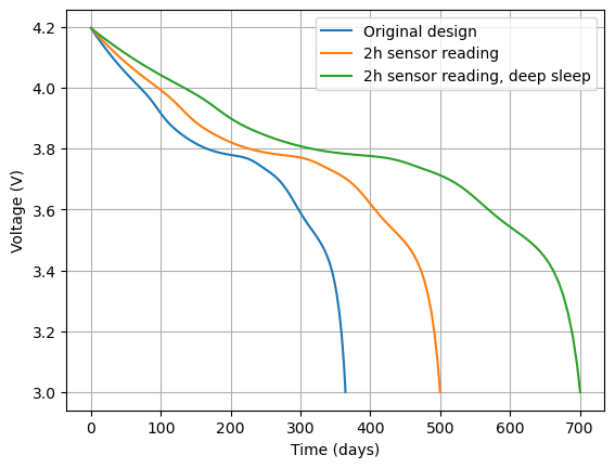
The battery life has now been extended to almost 700 days - quite an improvement.
Summary#
This tutorial explores the .batt_life() method in sysLoss for estimating battery life of the Bluetooth sensor system. Using callback functions sysLoss can integrate with just about any user supplied battery model, from ideal batteries to advanced chemistry models. sysLoss also identifies where the most energy is consumed, which makes system optimization for battery life much simpler.
References#
Python Battery Mathematical Modelling (PyBaMM): [SMT+21]